
All examples · Example 10 of 34
Box Plot: Western Blot Quantification
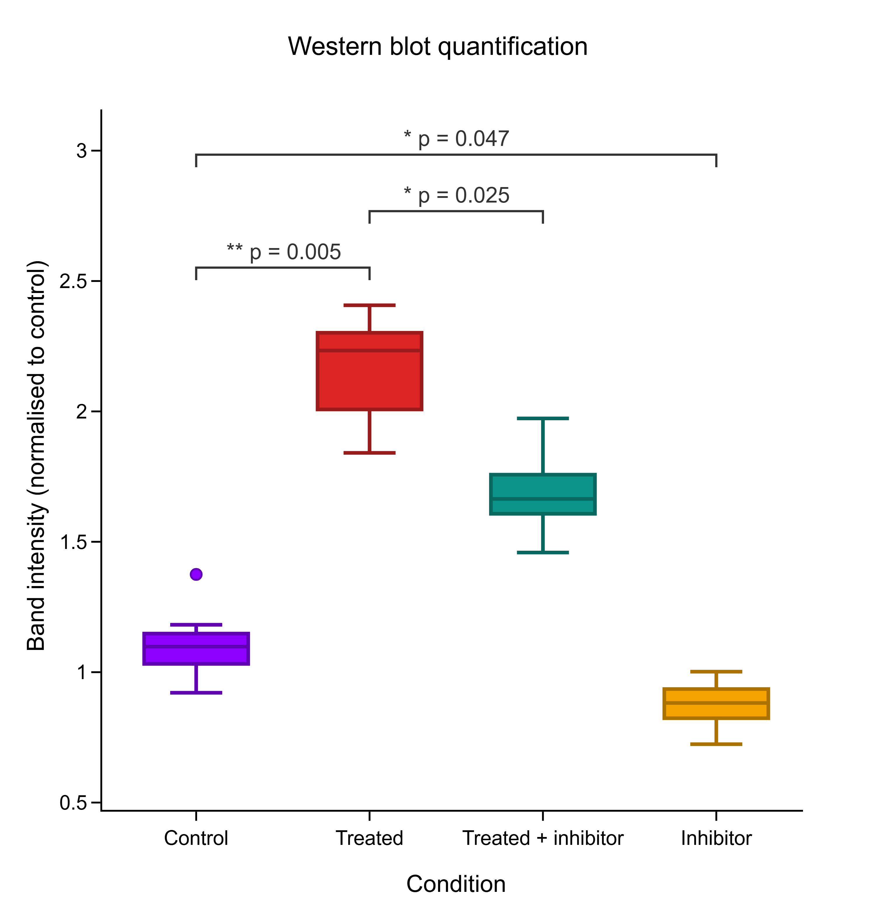
Normalised band intensity for four conditions (boxes: all 12 lanes per condition). Brackets show BH-adjusted Welch t-tests on biological-replicate means (n = 3).

Key findings
- Tested on biological-replicate means (n = 3 per condition), not on 12 lanes: the correct unit of analysis.
- One-way ANOVA F = 78.64, p = 2.8 × 10⁻⁶; Kruskal–Wallis p = 0.016. 6 of 6 Welch comparisons survive Holm correction.
- Rank tests hit a floor at this n: with 3 vs 3, Mann–Whitney cannot go below p = 0.081 even when the groups do not overlap at all (Cliff's δ = ±1), so none survives correction. With three replicates, only the parametric tests can reach significance.
- The minimum detectable effect at n = 3 per group is d = 3.07 (80% power): large effects like this treatment are visible, subtle ones would not be.
Design: why n = 3, not 12
Each condition has 3 biological replicates, each run as 4 technical lanes. Technical lanes are not independent — they share a lysate — so testing all 12 lanes as if they were would be pseudoreplication and would inflate every p-value. The lanes are averaged within each biological replicate (a mean computed here, before the data reach LabTools) and the tests below run on those n = 3 means per condition.
All lanes (descriptive only)
Per-condition summary of all 12 lanes. Useful for spotting a bad lane; not the unit of analysis.
| Group | n | Mean | SD | SEM | Median | Q1 – Q3 | Min – Max | Skewness | Excess kurtosis |
|---|---|---|---|---|---|---|---|---|---|
| Control | 12 | 1.097 | 0.1196 | 0.03451 | 1.098 | 1.037 – 1.145 | 0.921 – 1.375 | 0.773 | 1.95 |
| Treated | 12 | 2.169 | 0.1918 | 0.05537 | 2.234 | 2.029 – 2.28 | 1.841 – 2.407 | -0.611 | -0.898 |
| Treated + inhibitor | 12 | 1.673 | 0.1414 | 0.04083 | 1.664 | 1.618 – 1.741 | 1.459 – 1.973 | 0.437 | 0.829 |
| Inhibitor | 12 | 0.8764 | 0.08114 | 0.02342 | 0.882 | 0.8407 – 0.9333 | 0.724 – 1.002 | -0.425 | -0.336 |
LabTools call
stats.describelabtools stats describe --groups @groups.json
The same method is available as an MCP tool (stats_describe) and from the desktop app's statistics panel.
Lane-level outlier screen
Five detectors with different assumptions. Grubbs tests the single most extreme point, generalised ESD looks for up to several (immune to masking), Dixon's Q is the small-sample chemistry test, modified-z uses the median and MAD so needs no normality, and the IQR rule is Tukey's boxplot fence. LabTools flags points; it never deletes them.
| Method | Control | Treated | Treated + inhibitor | Inhibitor |
|---|---|---|---|---|
| Grubbs | none | none | none | none |
| Generalised ESD | none | none | none | none |
| Dixon's Q | none | none | none | none |
| Modified z (MAD) | none | none | none | none |
| IQR fences (1.5×) | 1 (1.375) | none | 1 (1.973) | none |
LabTools calls (5)
stats.outlierslabtools stats outliers --groups @groups.json --method grubbs
stats.outlierslabtools stats outliers --groups @groups.json --method generalized-esd --max-outliers 5
stats.outlierslabtools stats outliers --groups @groups.json --method dixon-q
stats.outlierslabtools stats outliers --groups @groups.json --method modified-z
stats.outlierslabtools stats outliers --groups @groups.json --method iqr
The same method is available as an MCP tool (stats_outliers) and from the desktop app's statistics panel.
LabTools notes
- Flagged points are candidates, not verdicts, and nothing has been removed. Look for a physical cause before excluding anything; if there is none, keep the point and use a robust test instead. Any exclusion must be reported.
- The IQR rule is descriptive — it has no p-value and flags roughly 0.7% of a perfectly normal sample by construction.
Biological-replicate means (the unit of analysis)
Location, spread and shape for every group — the first thing to read before choosing a test. Skewness near 0 and excess kurtosis near 0 are what a normal distribution looks like.
| Group | n | Mean | SD | SEM | Median | Q1 – Q3 | Min – Max | Skewness | Excess kurtosis |
|---|---|---|---|---|---|---|---|---|---|
| Control | 3 | 1.097 | 0.102 | 0.05889 | 1.097 | 1.046 – 1.148 | 0.9945 – 1.198 | -0.0221 | — |
| Treated | 3 | 2.169 | 0.165 | 0.09524 | 2.162 | 2.085 – 2.25 | 2.007 – 2.337 | 0.175 | — |
| Treated + inhibitor | 3 | 1.673 | 0.1101 | 0.06355 | 1.626 | 1.61 – 1.712 | 1.595 – 1.799 | 1.58 | — |
| Inhibitor | 3 | 0.8764 | 0.04633 | 0.02675 | 0.8732 | 0.8525 – 0.8987 | 0.8317 – 0.9243 | 0.306 | — |
LabTools call
stats.describelabtools stats describe --groups @groups.json
The same method is available as an MCP tool (stats_describe) and from the desktop app's statistics panel.
Equal variances
Student's t and one-way ANOVA assume every group has the same spread. LabTools' Levene test uses deviations from the group median (the Brown–Forsythe form), which stays reliable on skewed data; Bartlett's test is more powerful but only trustworthy when the data are normal. A significant p means the equal-variance assumption fails — prefer Welch's t-test or a rank-based test.
| Test | Statistic | p | Largest / smallest variance | Verdict |
|---|---|---|---|---|
| Levene (Brown–Forsythe, median-centred) | 0.5723 | 0.65 | 12.7 | Homogeneous |
| Bartlett | 2.228 | 0.53 | 12.7 | Homogeneous |
LabTools calls (2)
stats.levenelabtools stats levene --groups @groups.json --method levene
stats.levenelabtools stats levene --groups @groups.json --method bartlett
The same method is available as an MCP tool (stats_levene) and from the desktop app's statistics panel.
LabTools notes
- Group 'Control' has n = 3; normality screening has very low power at this size, so a non-significant Shapiro–Wilk is weak evidence of normality.
- Group 'Inhibitor' has n = 3; normality screening has very low power at this size, so a non-significant Shapiro–Wilk is weak evidence of normality.
- Group 'Treated' has n = 3; normality screening has very low power at this size, so a non-significant Shapiro–Wilk is weak evidence of normality.
- Group 'Treated + inhibitor' has n = 3; normality screening has very low power at this size, so a non-significant Shapiro–Wilk is weak evidence of normality.
- Non-significant. This test has low power on small samples, so treat this as 'no evidence against equal variances', not as evidence for them.
- Bartlett's test assumes normality and is badly inflated when that fails — confirm with stats.normality, or use method='levene'.
Do the groups differ? (omnibus tests)
One-way ANOVA compares means and assumes normal residuals with equal variances; Kruskal–Wallis compares ranks and assumes neither. Both only say the groups differ somewhere — the pairwise table below says where.
| Test | Statistic | df | p | Effect size |
|---|---|---|---|---|
| One-way ANOVA | F = 78.64 | 3, 8 | 2.8 × 10⁻⁶ | ω² = 0.951 · η² = 0.967 · Cohen's f = 5.43 |
| Kruskal–Wallis H | H = 10.38 | 3 | 0.016 | ε² = 0.944 |
LabTools calls (2)
stats.anovalabtools stats anova --groups @groups.json
stats.kruskallabtools stats kruskal --groups @groups.json
The same method is available as an MCP tool (stats_anova) and from the desktop app's statistics panel.
LabTools notes
- Group 'Control' has n = 3; normality screening has very low power at this size, so a non-significant Shapiro–Wilk is weak evidence of normality.
Which groups differ? (pairwise, corrected)
6 comparisons (every pair), each run as a Welch t-test and a Mann–Whitney test. Testing many pairs inflates false positives, so every p-value is corrected with Holm (family-wise) and Benjamini–Hochberg (false-discovery rate) through stats.adjust.
| Comparison | Mean diff. | 95% CI | Hedges' g | Welch p | Holm | BH | Mann–Whitney p | Holm | Cliff's δ |
|---|---|---|---|---|---|---|---|---|---|
| Control vs Treated | -1.072 | [-1.409, -0.7349] | -6.25 | 0.002 | 0.009 | 0.005 | 0.081 | 0.49 | -1 |
| Control vs Treated + inhibitor | -0.5764 | [-0.8175, -0.3353] | -4.35 | 0.003 | 0.011 | 0.005 | 0.081 | 0.49 | -1 |
| Control vs Inhibitor | 0.2203 | [0.005517, 0.4351] | 2.23 | 0.047 | 0.047 | 0.047 | 0.081 | 0.49 | 1 |
| Treated vs Treated + inhibitor | 0.4955 | [0.1582, 0.8328] | 2.83 | 0.017 | 0.033 | 0.020 | 0.081 | 0.49 | 1 |
| Treated vs Inhibitor | 1.292 | [0.9174, 1.667] | 8.53 | 0.003 | 0.011 | 0.005 | 0.081 | 0.49 | 1 |
| Treated + inhibitor vs Inhibitor | 0.7968 | [0.5621, 1.031] | 7.55 | 0.002 | 0.011 | 0.005 | 0.081 | 0.49 | 1 |
LabTools calls (3)
stats.ttestlabtools stats ttest --a @Control.json --b @Treated.json --test welch --no-assumption-checks
stats.mannwhitneylabtools stats mannwhitney --a @Control.json --b @Treated.json
stats.adjustlabtools stats adjust --p-values @p_values.json --labels @labels.json --method holm
The same method is available as an MCP tool (stats_ttest) and from the desktop app's statistics panel.
Design sensitivity
LabTools calls (2)
stats.powerlabtools stats power --n1 3 --n2 3 --mode mde --power 0.8
stats.powerlabtools stats power --n1 3 --n2 3 --effect-size 0.5
The same method is available as an MCP tool (stats_power) and from the desktop app's statistics panel.
Methods paragraph
Written to go straight into a manuscript.
To avoid pseudoreplication, technical replicates were averaged within each biological replicate and conditions compared by Welch’s t-test on the replicate means (n = 3); p-values were adjusted by Benjamini–Hochberg. Treatment increased band intensity 2.0-fold (p_adj = 0.005), and the inhibitor partially reversed it (p_adj = 0.025).
Every number on this page was computed by the LabTools statistics engine (version 0.14.3) from the example's CSV on 2026-09-23. Where a value was derived before the data reached LabTools (replicate means, paired differences, log odds ratios), the text says so. The data are simulated from a fixed random seed.
Get started
Run the same analysis on your data
Every test on this page is built into LabTools — from the statistics panel, the command line, or an AI assistant through MCP.