Histogram Distribution
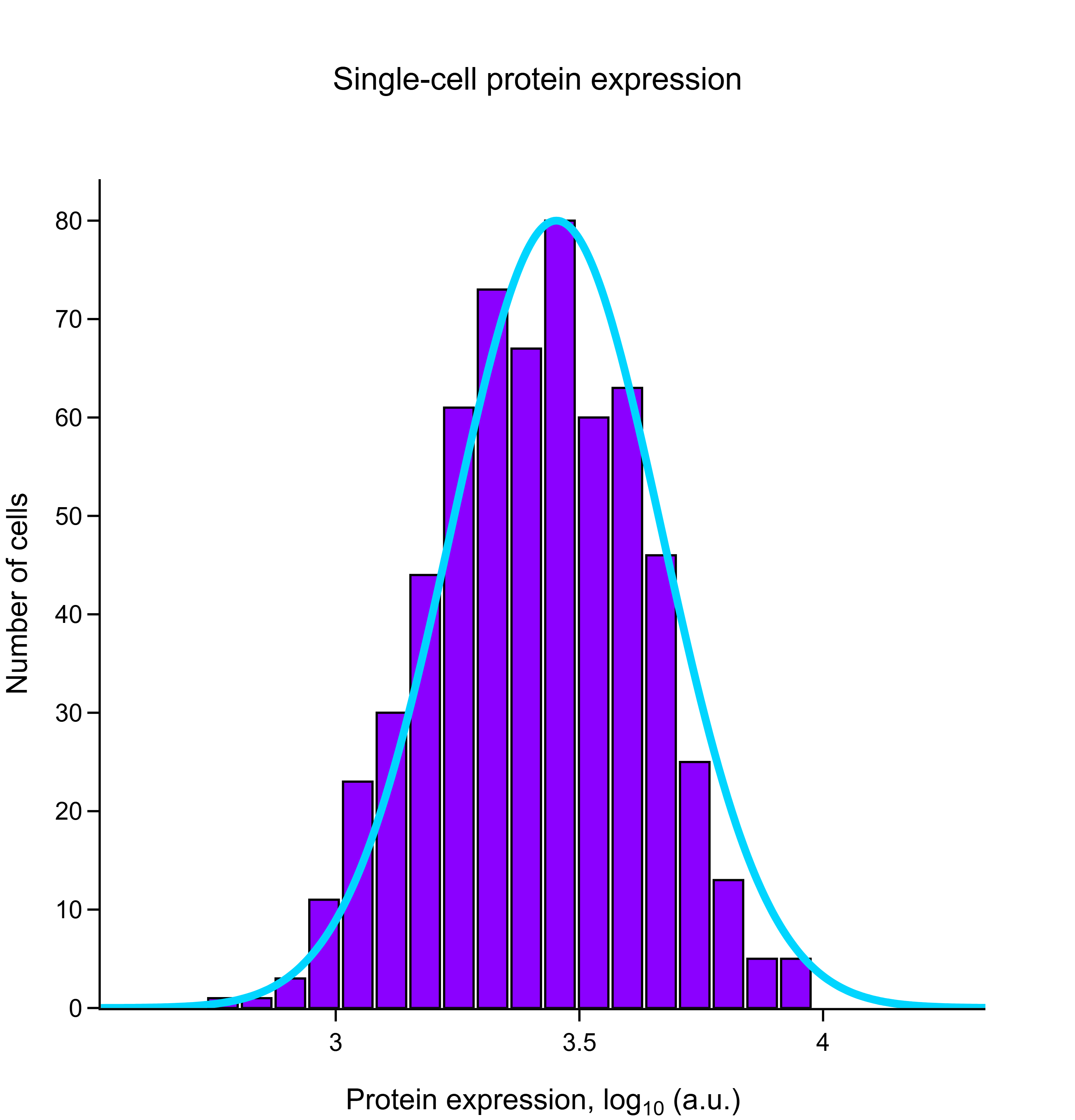
Protein Expression Histogram
Distribution of single-cell protein expression (log10 a.u.; n = 612 cells) with a fitted Gaussian (cyan).
Examples
34 chart types, each with a real use case and a full statistical report computed by the LabTools stats engine: assumption checks, parametric and rank-based tests, effect sizes, multiple-comparison corrections and power.
Showing 34 of 34 examples
Distribution of single-cell protein expression (log10 a.u.; n = 612 cells) with a fitted Gaussian (cyan).
DNA content per cell (n = 1,500) showing G1 (2N) and G2/M (4N) populations; Gaussian mixture components and their sum are overlaid.
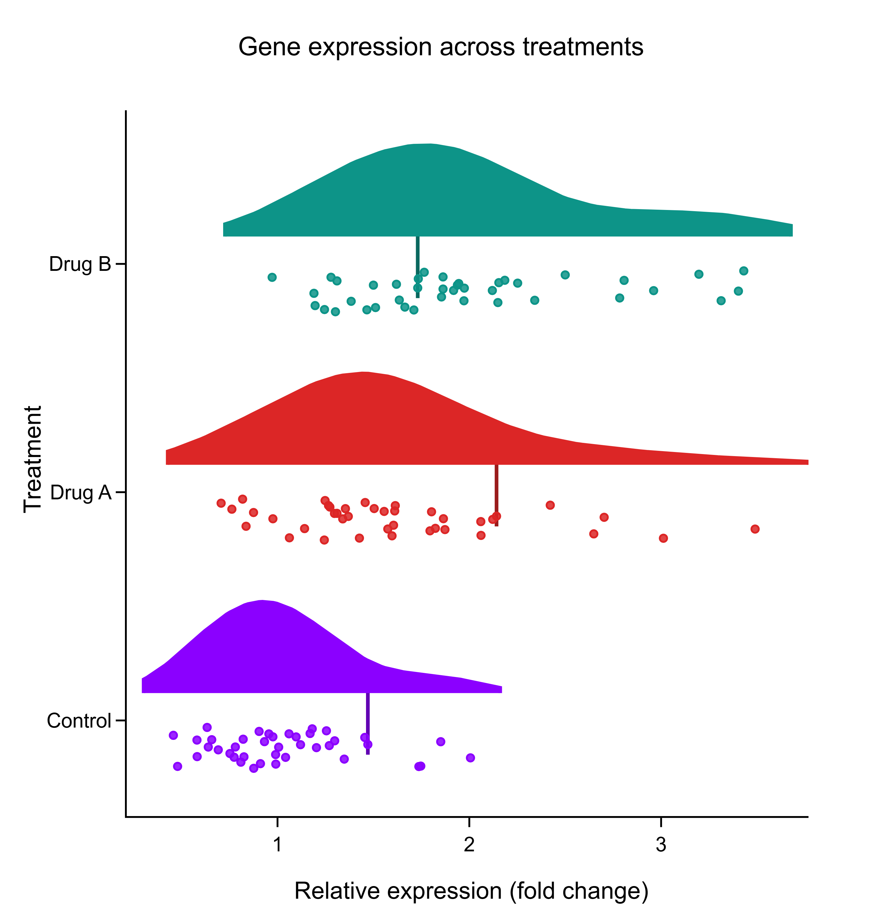
Relative expression of a target gene under three treatments (n = 40 per group): density (cloud), box plot and individual values (rain).
Cell viability (%) across five drug concentrations (n = 30 wells each); violins show the density with an inner IQR box and median.
Peak calcium transient amplitude (ΔF/F0) in individual WT and KO cells (n = 120 per genotype).
ΔCt (target − GAPDH) for each animal in four treatment groups (n = 8 per group); lower ΔCt means higher target expression.
Distribution of cell area (µm²) at eight time points after stimulation (n = 300 cells per time point).
Forward (FSC-A) vs side scatter (SSC-A) density for 20,000 events, showing two cell populations and low-scatter debris.
Normal Q–Q plot of 200 model residuals; points departing from the reference line at both ends indicate heavier tails than a normal distribution.
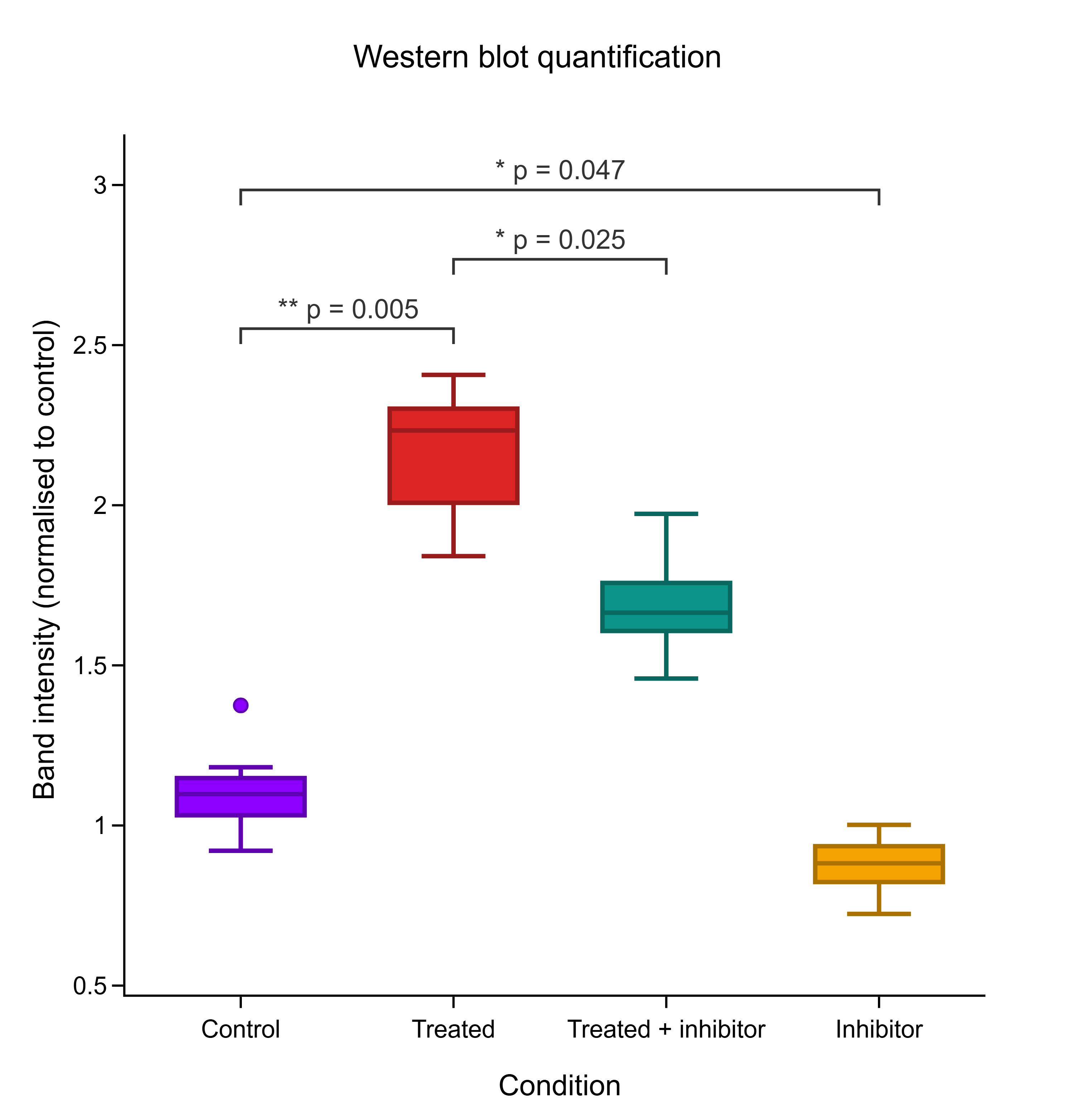
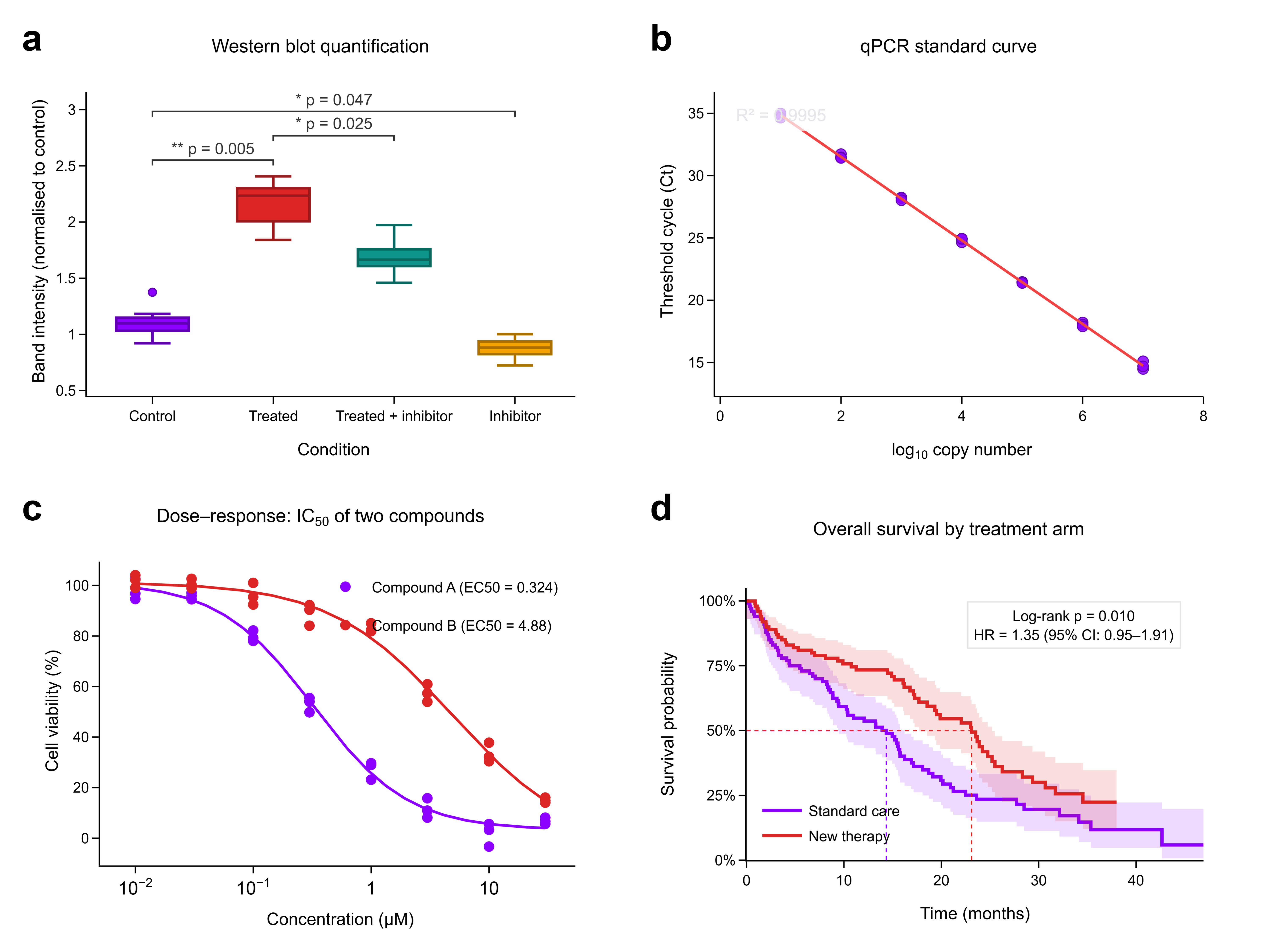
Normalised band intensity for four conditions (boxes: all 12 lanes per condition). Brackets show BH-adjusted Welch t-tests on biological-replicate means (n = 3).
Cytokine concentrations (pg/mL) in control and LPS-stimulated cultures; bars show mean ± SEM with individual wells (n = 6).
Best overall response (CR, PR, SD, PD) as a percentage of patients in each arm (n = 50 per arm).
Systolic blood pressure for each of 20 patients before and after treatment; lines join measurements from the same patient.
Best percentage change in tumour size from baseline for each of 30 patients, ordered from largest increase to largest decrease; dashed lines mark the RECIST +20% and −30% thresholds.
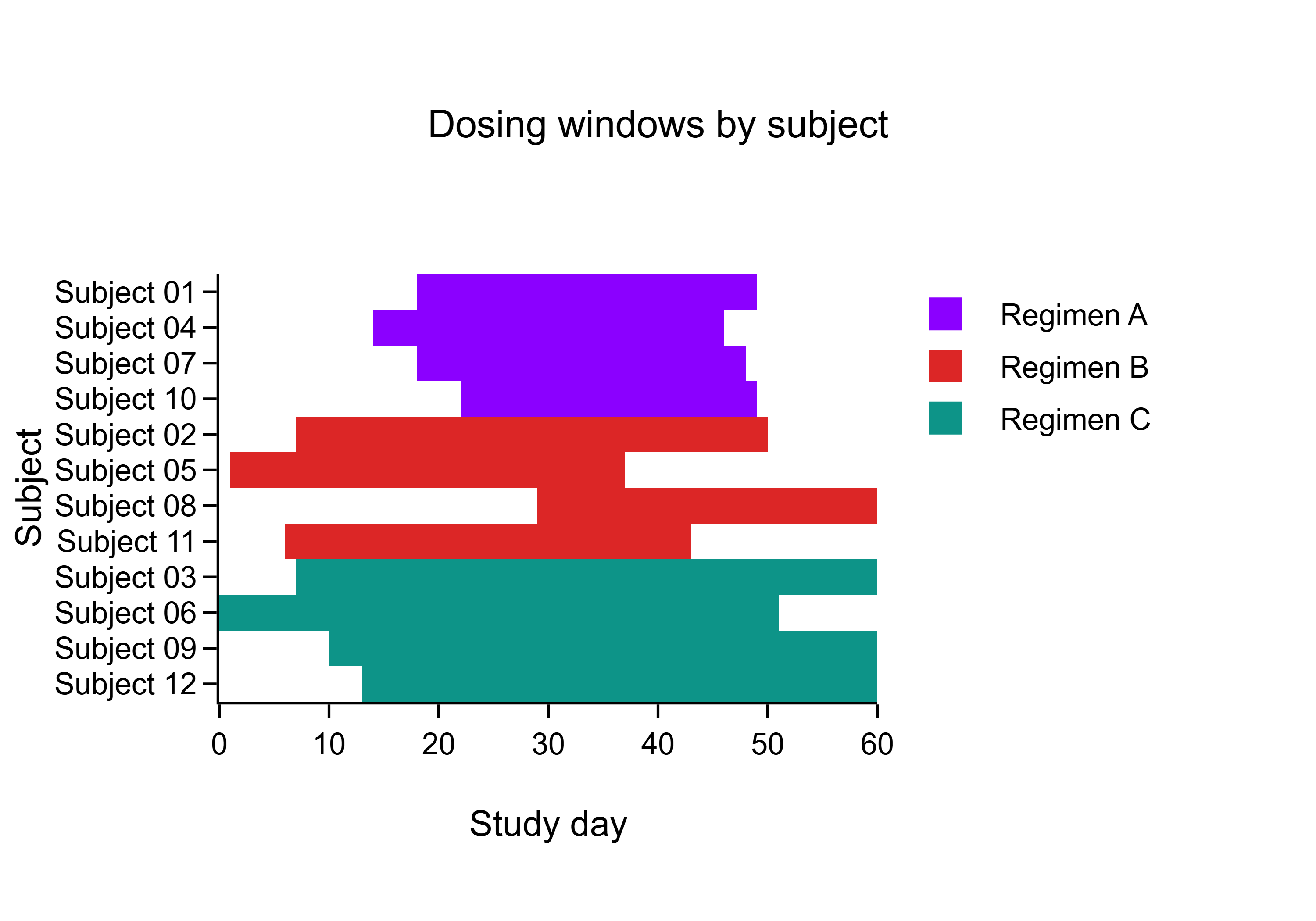
Dosing window (start to end study day) for each of 12 subjects, coloured by regimen.
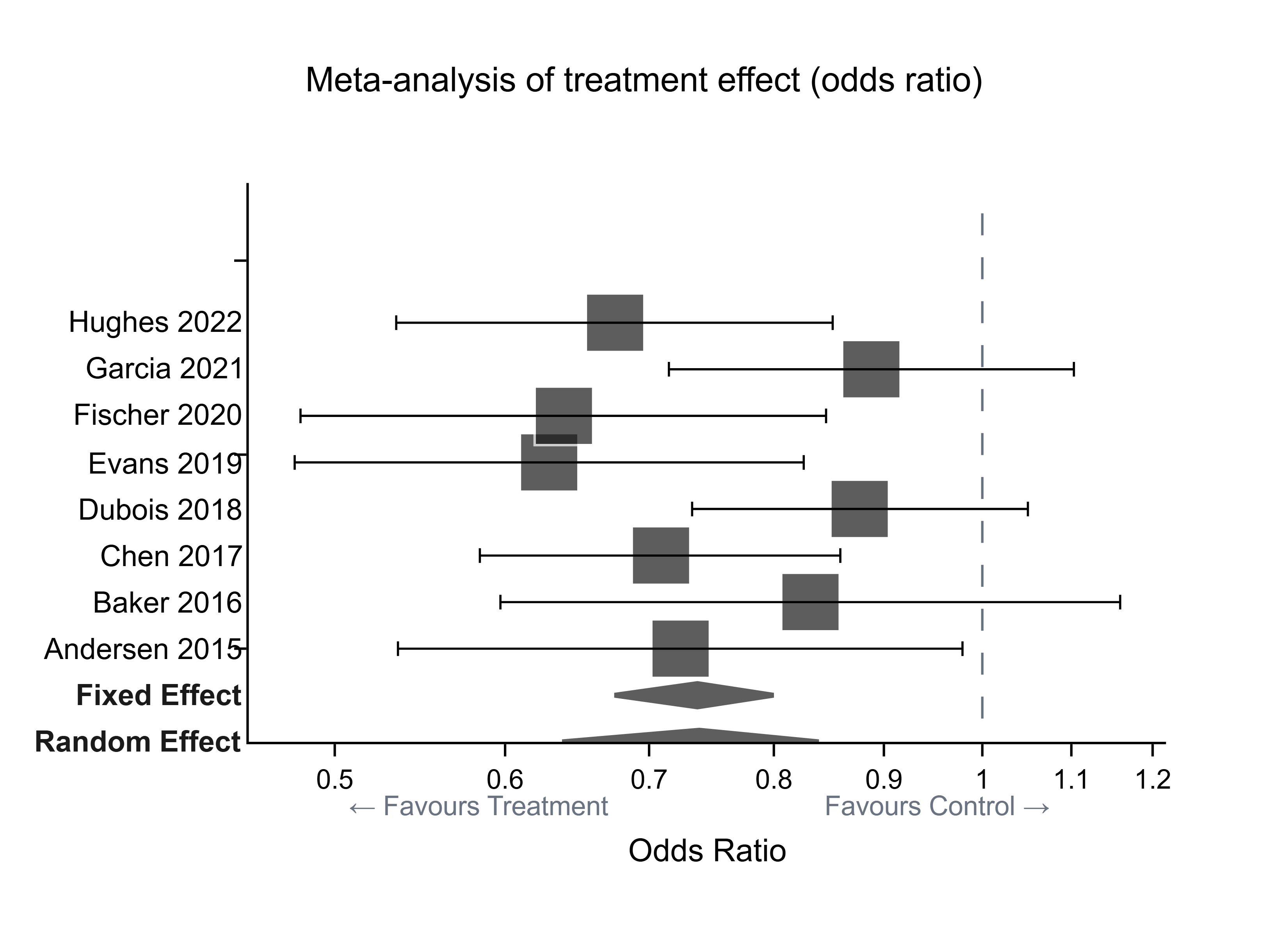
Odds ratios with 95% CIs from eight studies; diamonds show the fixed- and random-effect pooled estimates.
Threshold cycle (Ct) against log10 template copy number for a 7-point, 10-fold dilution series in triplicate, with the least-squares line.
Forty candidate biomarkers plotted by log2 fold change and −log10 p; dashed lines mark p = 0.05 and ±1 log2 fold change.
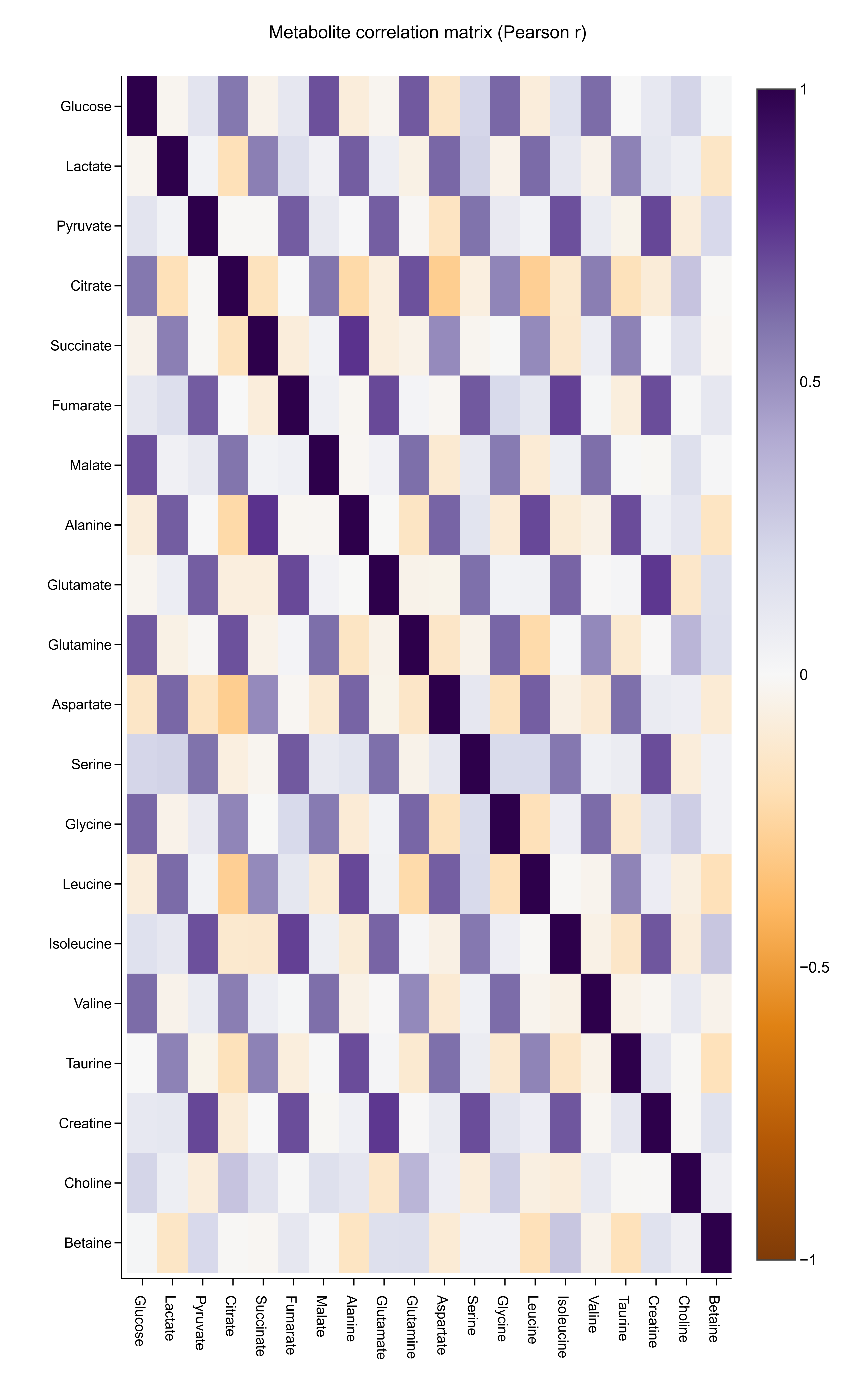
Pairwise Pearson correlation between 20 metabolites across 60 samples (purple positive, orange negative).
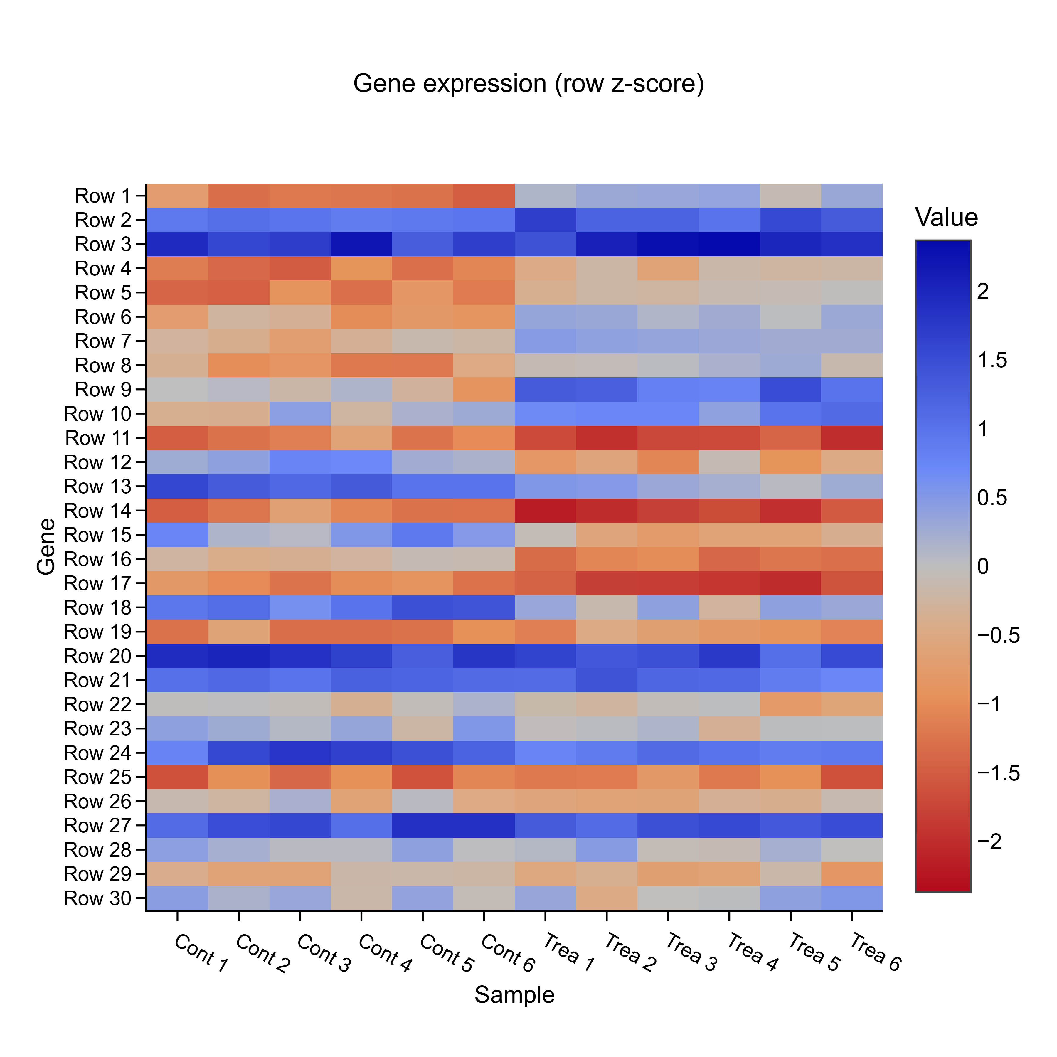
Row-standardised (z-score) log2 expression of 30 genes across 6 control and 6 treated samples.
Difference between point-of-care meter and reference analyser against their mean for 80 samples; solid line is the mean bias, dashed lines the 95% limits of agreement.
OD600 of bacterial cultures in three media over 24 h (mean ± SD of 3 replicate cultures).
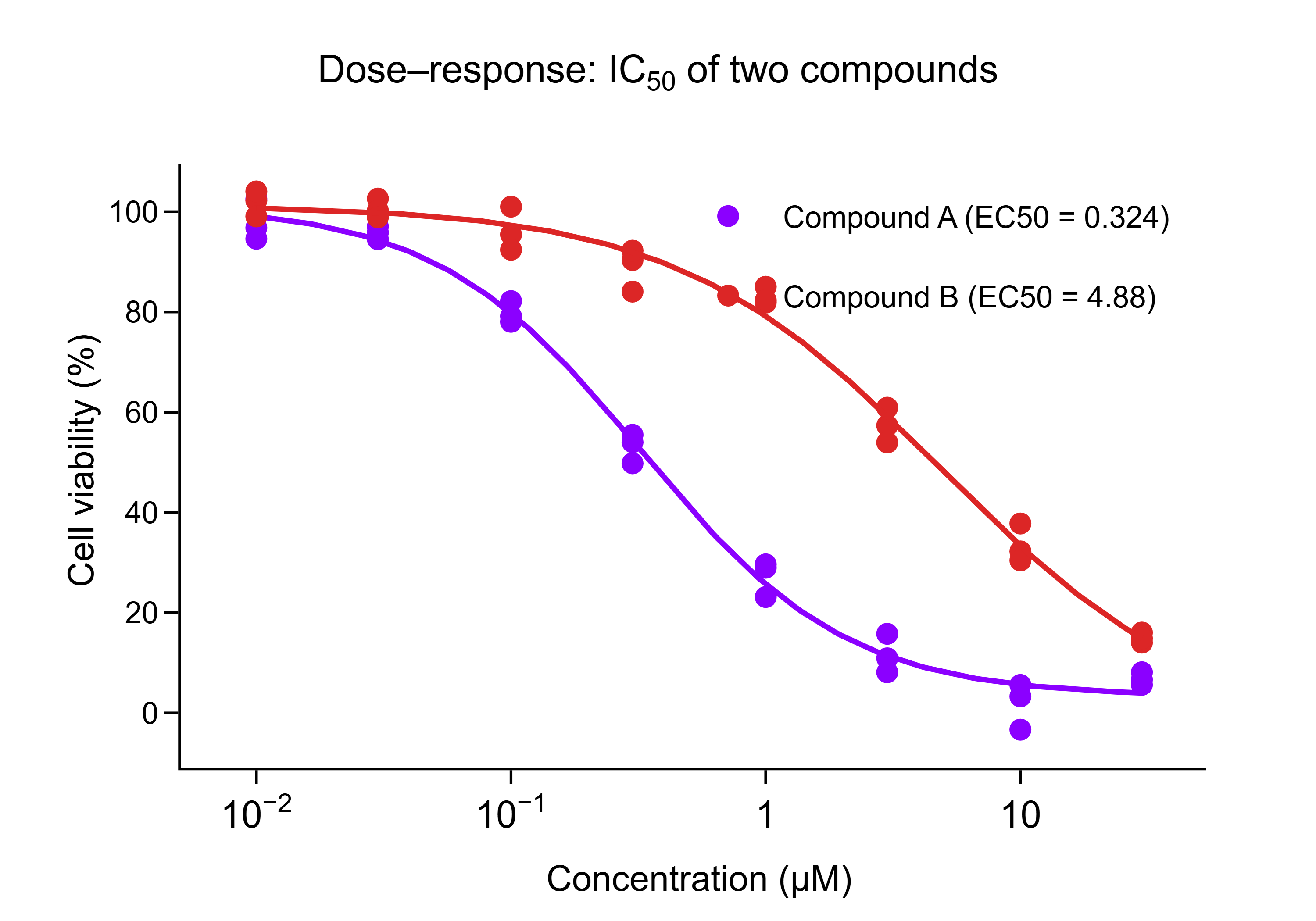
Cell viability against concentration for two compounds (triplicate wells) with four-parameter logistic fits.
Initial reaction velocity against substrate concentration (triplicates) with the fitted Michaelis–Menten curve.
Immune cell populations as a percentage of CD45+ leukocytes measured by flow cytometry.
Hierarchical breakdown of 15,740 immune cells: lineage (inner ring) and subset (outer ring).
Cell-type composition of five tissues; column width is proportional to cells sampled and segment height to the share of each cell type.
Kaplan–Meier overall survival for standard care and the new therapy (n = 100 per arm) with 95% confidence bands and censoring; dashed lines mark median survival.
Receiver operating characteristic curve for a biomarker score distinguishing 123 cases from 177 controls; dashed line is chance.
Differential expression of 8,000 genes: log2 fold change against −log10 adjusted p; red up-regulated, blue down-regulated.
Manhattan plot of 49,992 SNPs across 22 autosomes; the dashed line marks genome-wide significance (p = 5 × 10⁻⁸).
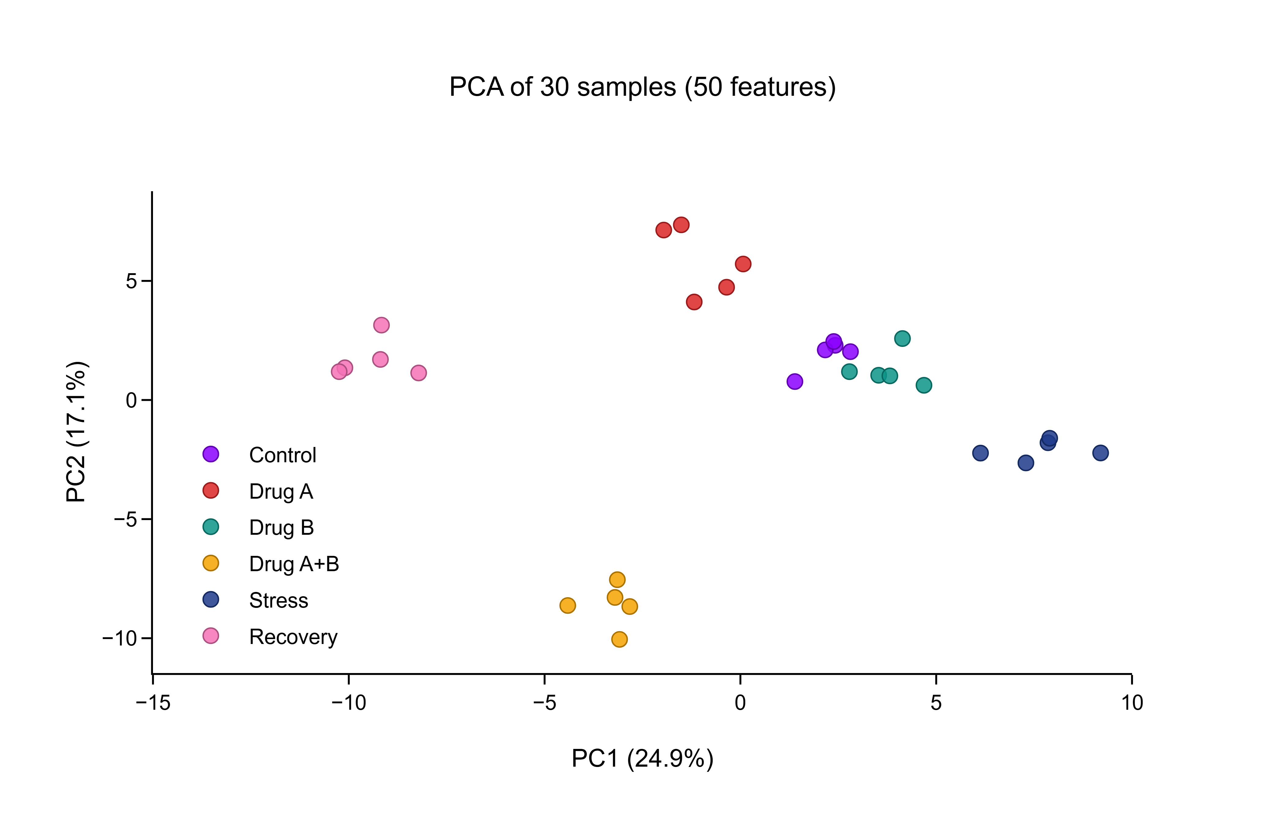
Principal component analysis of 30 samples (6 conditions × 5 replicates) on 50 features; points coloured by condition.
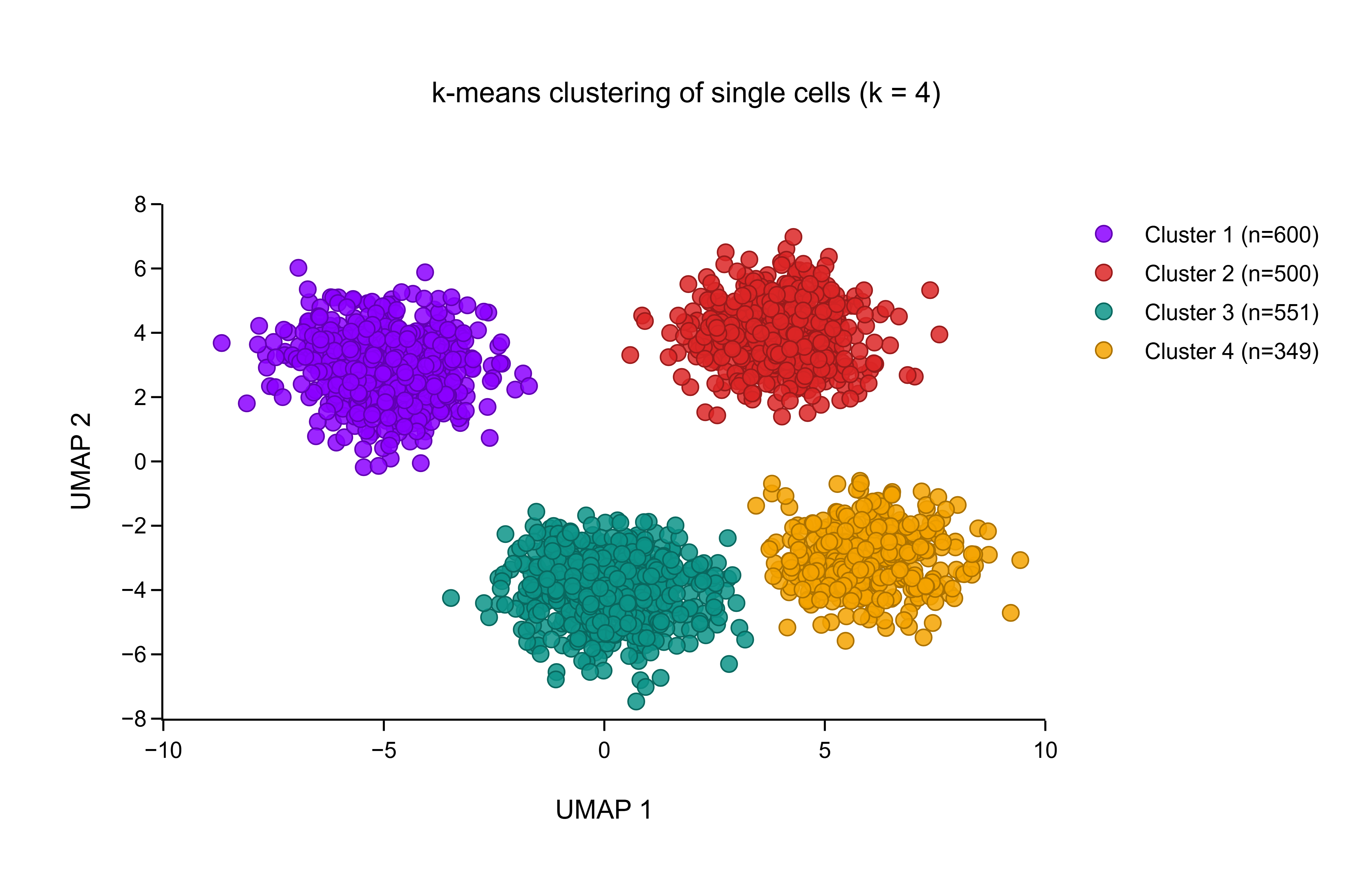
k-means clustering (k = 4) of 2,000 cells on a two-dimensional UMAP embedding.
A four-panel figure assembled in LabTools: (a) western blot quantification, (b) qPCR standard curve, (c) dose–response, (d) Kaplan–Meier survival.
Get started
Download LabTools and start generating figures like these in minutes.