
All examples · Example 3 of 34
Raincloud Plot: Gene Expression
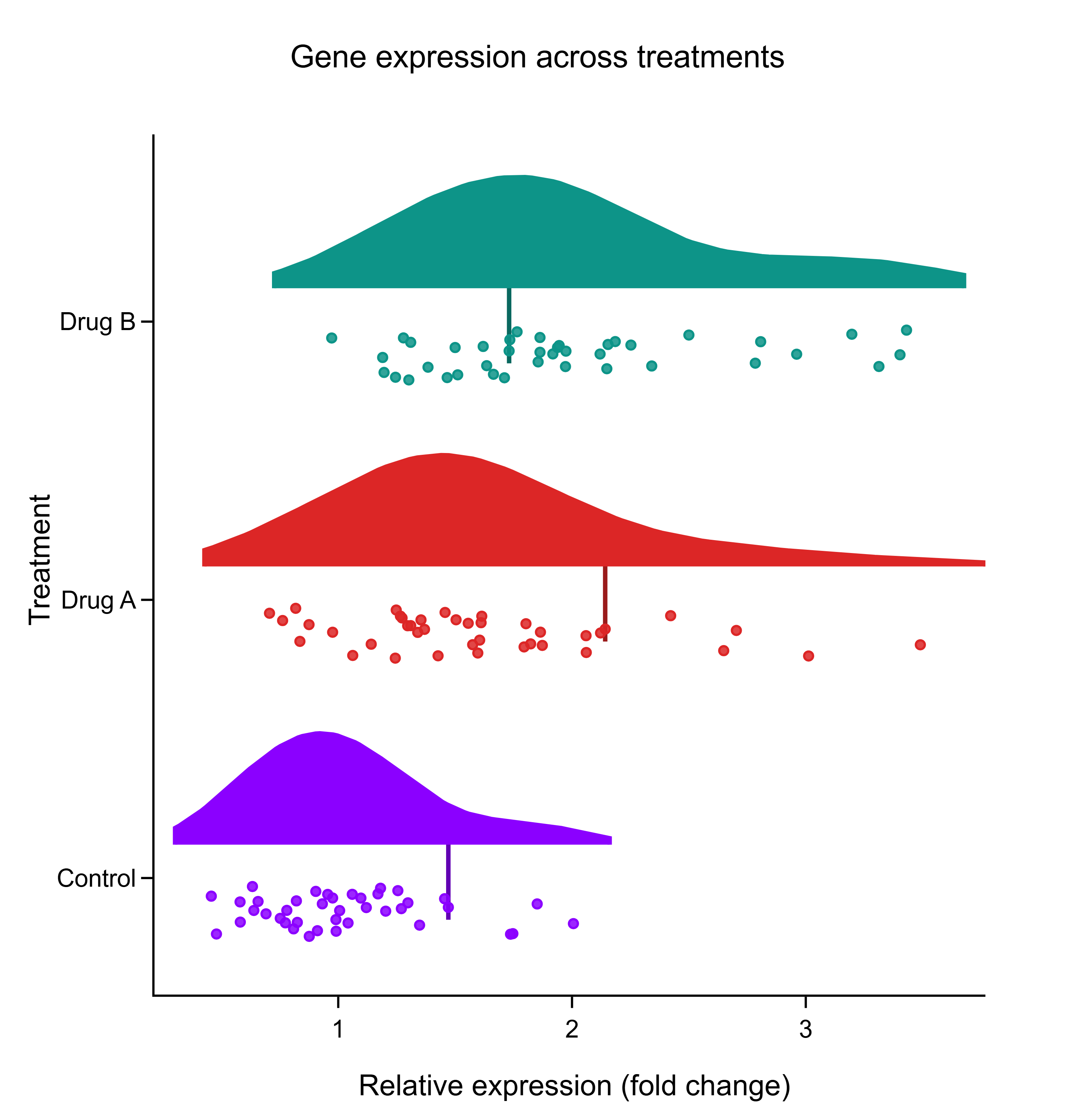
Relative expression of a target gene under three treatments (n = 40 per group): density (cloud), box plot and individual values (rain).

Key findings
- Kruskal–Wallis H = 47.61, p = 4.6 × 10⁻¹¹; one-way ANOVA agrees (F = 29.25, ω² = 0.32).
- All 3 pairwise differences survive Holm correction on both the Welch and the Mann–Whitney family.
- Levene's test flags unequal spread across groups, which is why Welch and rank-based tests are the ones to report.
Descriptive statistics
Location, spread and shape for every group — the first thing to read before choosing a test. Skewness near 0 and excess kurtosis near 0 are what a normal distribution looks like.
| Group | n | Mean | SD | SEM | Median | Q1 – Q3 | Min – Max | Skewness | Excess kurtosis |
|---|---|---|---|---|---|---|---|---|---|
| Control | 40 | 1.033 | 0.372 | 0.05883 | 0.983 | 0.7785 – 1.216 | 0.457 – 2.006 | 0.819 | 0.396 |
| Drug A | 40 | 1.616 | 0.6163 | 0.09745 | 1.53 | 1.262 – 1.867 | 0.706 – 3.49 | 1.05 | 1.32 |
| Drug B | 40 | 1.979 | 0.6441 | 0.1018 | 1.863 | 1.508 – 2.202 | 0.972 – 3.431 | 0.842 | 0.0464 |
LabTools call
stats.describelabtools stats describe --groups @groups.json
The same method is available as an MCP tool (stats_describe) and from the desktop app's statistics panel.
Normality
Three tests of the same question — could these values come from a normal distribution? Shapiro–Wilk has the best power at bench sample sizes, Anderson–Darling is more sensitive in the tails, and Kolmogorov–Smirnov (Lilliefors-corrected) is included for comparability with older papers. A significant p means normality is rejected.
| Group | n | Shapiro–Wilk W | p | Anderson–Darling A² | p | K–S D | p | Verdict |
|---|---|---|---|---|---|---|---|---|
| Control | 40 | 0.9469 | 0.059 | 0.6093 | 0.11 | 0.1042 | 0.34 | Consistent with normal |
| Drug A | 40 | 0.9304 | 0.017 | 0.8063 | 0.034 | 0.1513 | 0.022 | Normality rejected |
| Drug B | 40 | 0.9226 | 0.009 | 1.025 | 0.009 | 0.1528 | 0.020 | Normality rejected |
LabTools calls (3)
stats.normalitylabtools stats normality --groups @groups.json --method shapiro-wilk
stats.normalitylabtools stats normality --groups @groups.json --method anderson-darling
stats.normalitylabtools stats normality --groups @groups.json --method kolmogorov-smirnov
The same method is available as an MCP tool (stats_normality) and from the desktop app's statistics panel.
LabTools notes
- Group 'Drug A' rejects normality (p = 0.0166); prefer a rank-based test.
- Group 'Drug B' rejects normality (p = 0.0093); prefer a rank-based test.
- Group 'Drug A' rejects normality (p = 0.0337); prefer a rank-based test.
- Group 'Drug B' rejects normality (p = 0.0095); prefer a rank-based test.
- Group 'Drug A' rejects normality (p = 0.0217); prefer a rank-based test.
- Group 'Drug B' rejects normality (p = 0.0195); prefer a rank-based test.
Equal variances
Student's t and one-way ANOVA assume every group has the same spread. LabTools' Levene test uses deviations from the group median (the Brown–Forsythe form), which stays reliable on skewed data; Bartlett's test is more powerful but only trustworthy when the data are normal. A significant p means the equal-variance assumption fails — prefer Welch's t-test or a rank-based test.
| Test | Statistic | p | Largest / smallest variance | Verdict |
|---|---|---|---|---|
| Levene (Brown–Forsythe, median-centred) | 3.288 | 0.041 | 3 | Variances differ |
| Bartlett | 12.41 | 0.002 | 3 | Variances differ |
LabTools calls (2)
stats.levenelabtools stats levene --groups @groups.json --method levene
stats.levenelabtools stats levene --groups @groups.json --method bartlett
The same method is available as an MCP tool (stats_levene) and from the desktop app's statistics panel.
LabTools notes
- Variances differ: use Welch's t-test (stats.ttest default) or stats.kruskal rather than the pooled-variance alternatives.
- Bartlett's test assumes normality and is badly inflated when that fails — confirm with stats.normality, or use method='levene'.
Outlier screen
Five detectors with different assumptions. Grubbs tests the single most extreme point, generalised ESD looks for up to several (immune to masking), Dixon's Q is the small-sample chemistry test, modified-z uses the median and MAD so needs no normality, and the IQR rule is Tukey's boxplot fence. LabTools flags points; it never deletes them.
| Method | Control | Drug A | Drug B |
|---|---|---|---|
| Grubbs | none | 1 (3.49) | none |
| Generalised ESD | none | 1 (3.49) | none |
| Modified z (MAD) | none | 1 (3.49) | none |
| IQR fences (1.5×) | 1 (2.006) | 2 (3.012, 3.49) | 3 (3.431, 3.403, 3.313) |
LabTools calls (4)
stats.outlierslabtools stats outliers --groups @groups.json --method grubbs
stats.outlierslabtools stats outliers --groups @groups.json --method generalized-esd --max-outliers 5
stats.outlierslabtools stats outliers --groups @groups.json --method modified-z
stats.outlierslabtools stats outliers --groups @groups.json --method iqr
The same method is available as an MCP tool (stats_outliers) and from the desktop app's statistics panel.
LabTools notes
- Flagged points are candidates, not verdicts, and nothing has been removed. Look for a physical cause before excluding anything; if there is none, keep the point and use a robust test instead. Any exclusion must be reported.
- Grubbs tests only the single most extreme point, so a second outlier can mask the first. On larger samples use method='generalized_esd'.
- The IQR rule is descriptive — it has no p-value and flags roughly 0.7% of a perfectly normal sample by construction.
Confidence intervals for the mean
t-based intervals: the range of population means these data are consistent with. Report them alongside p-values — an interval shows the size of an effect, a p-value does not.
| Group | n | Mean | 95% CI |
|---|---|---|---|
| Control | 40 | 1.033 | [0.9143, 1.152] |
| Drug A | 40 | 1.616 | [1.419, 1.813] |
| Drug B | 40 | 1.979 | [1.773, 2.184] |
LabTools calls (2)
stats.cilabtools stats ci --data @Control.json --conf-level 0.95
stats.cilabtools stats ci --data @Drug_B.json --conf-level 0.95
The same method is available as an MCP tool (stats_ci) and from the desktop app's statistics panel.
Do the groups differ? (omnibus tests)
One-way ANOVA compares means and assumes normal residuals with equal variances; Kruskal–Wallis compares ranks and assumes neither. Both only say the groups differ somewhere — the pairwise table below says where.
| Test | Statistic | df | p | Effect size |
|---|---|---|---|---|
| One-way ANOVA | F = 29.25 | 2, 117 | 5.0 × 10⁻¹¹ | ω² = 0.32 · η² = 0.333 · Cohen's f = 0.707 |
| Kruskal–Wallis H | H = 47.61 | 2 | 4.6 × 10⁻¹¹ | ε² = 0.4 |
LabTools calls (2)
stats.anovalabtools stats anova --groups @groups.json
stats.kruskallabtools stats kruskal --groups @groups.json
The same method is available as an MCP tool (stats_anova) and from the desktop app's statistics panel.
LabTools notes
- Group 'Drug A' departs from normality (Shapiro–Wilk W = 0.9304, p = 0.0166 < 0.05). Consider stats.kruskal.
- Group 'Drug B' departs from normality (Shapiro–Wilk W = 0.9226, p = 0.0093 < 0.05). Consider stats.kruskal.
- Group variances are unequal (Levene W = 3.2876, p = 0.0408 < 0.05); the equal-variance assumption of this test is violated. Use the Welch variant instead.
Which groups differ? (pairwise, corrected)
3 comparisons (every pair), each run as a Welch t-test and a Mann–Whitney test. Testing many pairs inflates false positives, so every p-value is corrected with Holm (family-wise) and Benjamini–Hochberg (false-discovery rate) through stats.adjust.
| Comparison | Mean diff. | 95% CI | Hedges' g | Welch p | Holm | BH | Mann–Whitney p | Holm | Cliff's δ |
|---|---|---|---|---|---|---|---|---|---|
| Control vs Drug A | -0.5828 | [-0.8102, -0.3554] | -1.13 | 3.0 × 10⁻⁶ | 6.0 × 10⁻⁶ | 4.5 × 10⁻⁶ | 2.4 × 10⁻⁶ | 4.8 × 10⁻⁶ | -0.613 |
| Control vs Drug B | -0.9453 | [-1.18, -0.7102] | -1.78 | 3.3 × 10⁻¹¹ | 9.8 × 10⁻¹¹ | 9.8 × 10⁻¹¹ | 1.0 × 10⁻¹⁰ | 3.1 × 10⁻¹⁰ | -0.84 |
| Drug A vs Drug B | -0.3624 | [-0.643, -0.0818] | -0.569 | 0.012 | 0.012 | 0.012 | 0.007 | 0.007 | -0.352 |
LabTools calls (3)
stats.ttestlabtools stats ttest --a @Control.json --b @Drug_A.json --test welch --no-assumption-checks
stats.mannwhitneylabtools stats mannwhitney --a @Control.json --b @Drug_A.json
stats.adjustlabtools stats adjust --p-values @p_values.json --labels @labels.json --method holm
The same method is available as an MCP tool (stats_ttest) and from the desktop app's statistics panel.
Design sensitivity
LabTools calls (2)
stats.powerlabtools stats power --n1 40 --n2 40 --mode mde --power 0.8
stats.powerlabtools stats power --n1 40 --n2 40 --effect-size 0.5
The same method is available as an MCP tool (stats_power) and from the desktop app's statistics panel.
Methods paragraph
Written to go straight into a manuscript.
Groups were compared by Kruskal–Wallis (H = 47.6, df = 2, p < 0.0001, ε² = 0.40), followed by pairwise Mann–Whitney U tests with Holm correction; all pairs differed (adjusted p ≤ 0.007).
Every number on this page was computed by the LabTools statistics engine (version 0.14.3) from the example's CSV on 2026-09-23. Where a value was derived before the data reached LabTools (replicate means, paired differences, log odds ratios), the text says so. The data are simulated from a fixed random seed.
Get started
Run the same analysis on your data
Every test on this page is built into LabTools — from the statistics panel, the command line, or an AI assistant through MCP.