
All examples · Example 32 of 34
PCA: Sample Clustering
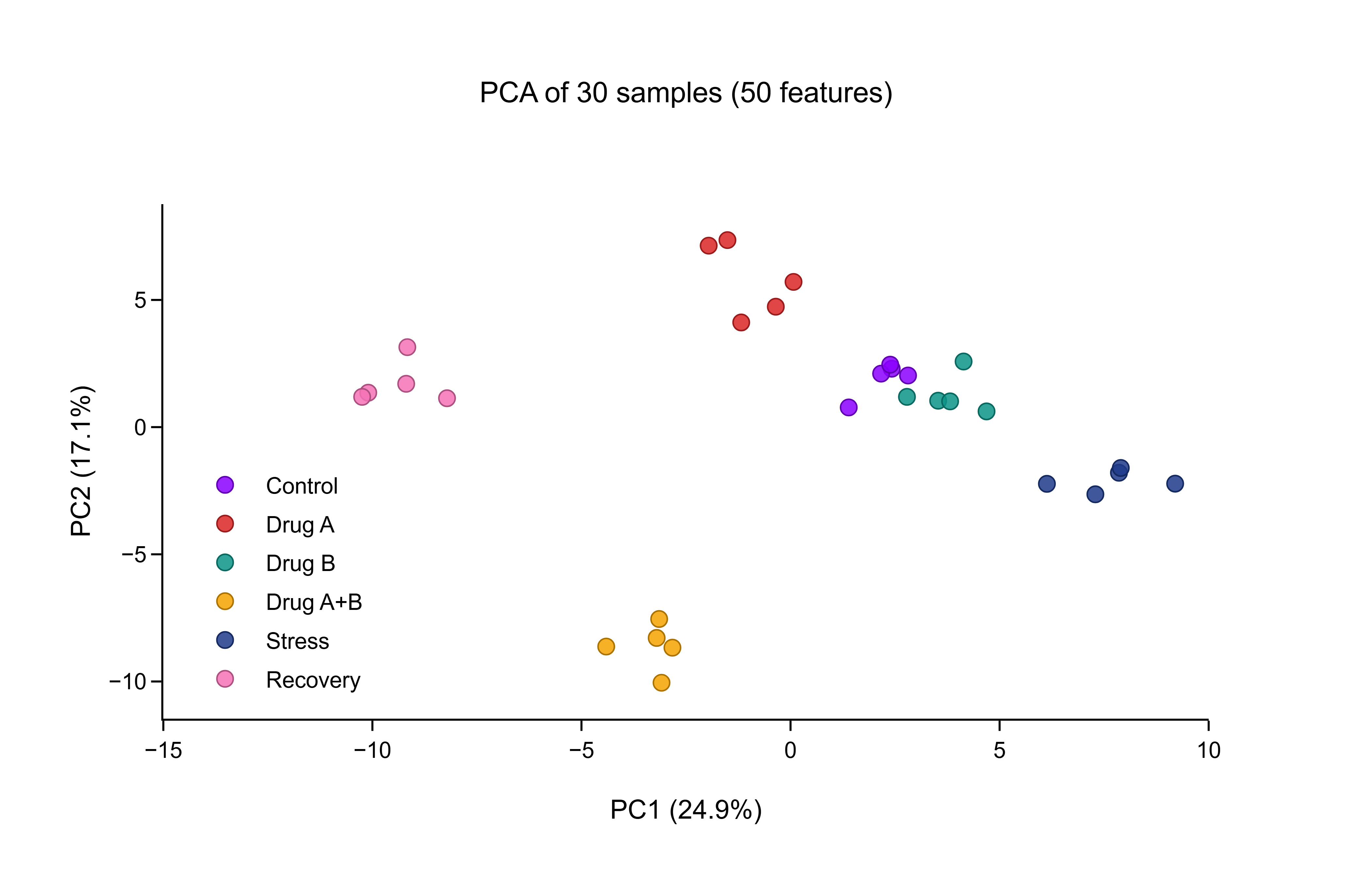
Principal component analysis of 30 samples (6 conditions × 5 replicates) on 50 features; points coloured by condition.

Key findings
- PC1 and PC2 explain 24.9% and 17.1% of the variance.
- 48 of 50 features differ between conditions after Benjamini–Hochberg correction (43 after Bonferroni); the strongest is Feature39 (ω² = 0.892).
Which of the 50 features separate the conditions?
PCA shows that the 6 conditions separate; this asks which features drive it. Each feature gets a one-way ANOVA across the conditions (n = 5 samples each), and the 50 p-values are corrected as one family.
50 tests, α = 0.05
| Correction | Controls | Tests | Raw p < 0.05 | Significant after correction |
|---|---|---|---|---|
| Bonferroni | family-wise error | 50 | 48 | 43 |
| Holm | family-wise error | 50 | 48 | 47 |
| Benjamini–Hochberg | false discovery rate | 50 | 48 | 48 |
| Benjamini–Yekutieli | false discovery rate | 50 | 48 | 47 |
LabTools calls (5)
stats.anovalabtools stats anova --groups @Feature01.json --no-assumption-checks
stats.adjustlabtools stats adjust --p-values @p_values.json --labels @labels.json --method bonferroni --alpha 0.05
stats.adjustlabtools stats adjust --p-values @p_values.json --labels @labels.json --method holm --alpha 0.05
stats.adjustlabtools stats adjust --p-values @p_values.json --labels @labels.json --method benjamini-hochberg --alpha 0.05
stats.adjustlabtools stats adjust --p-values @p_values.json --labels @labels.json --method benjamini-yekutieli --alpha 0.05
The same method is available as an MCP tool (stats_anova) and from the desktop app's statistics panel.
Top 15 by raw p
| Feature | F | ω² | Raw p | Bonferroni | Holm | BH | BY |
|---|---|---|---|---|---|---|---|
| Feature39 | 50.45 | 0.892 | 5.9 × 10⁻¹² | 3.0 × 10⁻¹⁰ | 3.0 × 10⁻¹⁰ | 3.0 × 10⁻¹⁰ | 1.3 × 10⁻⁹ |
| Feature11 | 44.74 | 0.879 | 2.2 × 10⁻¹¹ | 1.1 × 10⁻⁹ | 1.1 × 10⁻⁹ | 5.3 × 10⁻¹⁰ | 2.4 × 10⁻⁹ |
| Feature16 | 43.13 | 0.875 | 3.2 × 10⁻¹¹ | 1.6 × 10⁻⁹ | 1.5 × 10⁻⁹ | 5.3 × 10⁻¹⁰ | 2.4 × 10⁻⁹ |
| Feature31 | 40.29 | 0.868 | 6.6 × 10⁻¹¹ | 3.3 × 10⁻⁹ | 3.1 × 10⁻⁹ | 8.2 × 10⁻¹⁰ | 3.7 × 10⁻⁹ |
| Feature25 | 36.52 | 0.855 | 1.8 × 10⁻¹⁰ | 9.2 × 10⁻⁹ | 8.5 × 10⁻⁹ | 1.8 × 10⁻⁹ | 8.0 × 10⁻⁹ |
| Feature32 | 36.02 | 0.854 | 2.1 × 10⁻¹⁰ | 1.1 × 10⁻⁸ | 9.6 × 10⁻⁹ | 1.8 × 10⁻⁹ | 8.0 × 10⁻⁹ |
| Feature18 | 34.3 | 0.847 | 3.5 × 10⁻¹⁰ | 1.8 × 10⁻⁸ | 1.6 × 10⁻⁸ | 2.5 × 10⁻⁹ | 1.1 × 10⁻⁸ |
| Feature10 | 32.98 | 0.842 | 5.3 × 10⁻¹⁰ | 2.7 × 10⁻⁸ | 2.3 × 10⁻⁸ | 3.3 × 10⁻⁹ | 1.5 × 10⁻⁸ |
| Feature15 | 32.02 | 0.838 | 7.2 × 10⁻¹⁰ | 3.6 × 10⁻⁸ | 3.0 × 10⁻⁸ | 4.0 × 10⁻⁹ | 1.8 × 10⁻⁸ |
| Feature40 | 31.67 | 0.836 | 8.1 × 10⁻¹⁰ | 4.0 × 10⁻⁸ | 3.3 × 10⁻⁸ | 4.0 × 10⁻⁹ | 1.8 × 10⁻⁸ |
| Feature41 | 31.21 | 0.834 | 9.4 × 10⁻¹⁰ | 4.7 × 10⁻⁸ | 3.8 × 10⁻⁸ | 4.3 × 10⁻⁹ | 1.9 × 10⁻⁸ |
| Feature13 | 27.45 | 0.815 | 3.4 × 10⁻⁹ | 1.7 × 10⁻⁷ | 1.3 × 10⁻⁷ | 1.4 × 10⁻⁸ | 6.4 × 10⁻⁸ |
| Feature34 | 26.09 | 0.807 | 5.7 × 10⁻⁹ | 2.8 × 10⁻⁷ | 2.2 × 10⁻⁷ | 2.2 × 10⁻⁸ | 9.9 × 10⁻⁸ |
| Feature44 | 25.54 | 0.804 | 7.0 × 10⁻⁹ | 3.5 × 10⁻⁷ | 2.6 × 10⁻⁷ | 2.5 × 10⁻⁸ | 1.1 × 10⁻⁷ |
| Feature45 | 21.63 | 0.775 | 3.5 × 10⁻⁸ | 1.8 × 10⁻⁶ | 1.3 × 10⁻⁶ | 1.2 × 10⁻⁷ | 5.3 × 10⁻⁷ |
LabTools notes
- 5 comparison(s) were significant on the raw p-values but are not after correction. Report the adjusted values.
- Holm controls the same familywise error rate as Bonferroni and rejects at least as much, so there is no statistical reason to prefer bonferroni.
- 1 comparison(s) were significant on the raw p-values but are not after correction. Report the adjusted values.
Top feature: Feature39
Location, spread and shape for every group — the first thing to read before choosing a test. Skewness near 0 and excess kurtosis near 0 are what a normal distribution looks like.
| Group | n | Mean | SD | SEM | Median | Q1 – Q3 | Min – Max | Skewness | Excess kurtosis |
|---|---|---|---|---|---|---|---|---|---|
| Control | 5 | 1.878 | 0.6674 | 0.2985 | 1.702 | 1.35 – 2.327 | 1.22 – 2.793 | 0.584 | -1.65 |
| Drug A | 5 | -1.656 | 1.02 | 0.4562 | -1.334 | -1.668 – -1.27 | -3.359 – -0.651 | -1.5 | 2.91 |
| Drug B | 5 | 0.208 | 0.9924 | 0.4438 | 0.095 | -0.24 – 0.378 | -0.942 – 1.749 | 0.875 | 1.57 |
| Drug A+B | 5 | -4.927 | 0.7578 | 0.3389 | -5.009 | -5.075 – -4.463 | -6.05 – -4.037 | -0.59 | 0.585 |
| Stress | 5 | 2.747 | 1.165 | 0.5209 | 2.453 | 1.995 – 2.983 | 1.671 – 4.634 | 1.33 | 1.74 |
| Recovery | 5 | -2.626 | 0.7574 | 0.3387 | -2.538 | -2.897 – -2.056 | -3.771 – -1.866 | -0.862 | 0.223 |
LabTools call
stats.describelabtools stats describe --groups @groups.json
The same method is available as an MCP tool (stats_describe) and from the desktop app's statistics panel.
Feature39: which conditions differ?
One-way ANOVA compares means and assumes normal residuals with equal variances; Kruskal–Wallis compares ranks and assumes neither. Both only say the groups differ somewhere — the pairwise table below says where.
| Test | Statistic | df | p | Effect size |
|---|---|---|---|---|
| One-way ANOVA | F = 50.45 | 5, 24 | 5.9 × 10⁻¹² | ω² = 0.892 · η² = 0.913 · Cohen's f = 3.24 |
| Kruskal–Wallis H | H = 26.4 | 5 | 7.5 × 10⁻⁵ | ε² = 0.91 |
LabTools calls (2)
stats.anovalabtools stats anova --groups @groups.json
stats.kruskallabtools stats kruskal --groups @groups.json
The same method is available as an MCP tool (stats_anova) and from the desktop app's statistics panel.
LabTools notes
- Group 'Control' has n = 5; normality screening has very low power at this size, so a non-significant Shapiro–Wilk is weak evidence of normality.
Which groups differ? (pairwise, corrected)
5 comparisons (each group against Control), each run as a Welch t-test and a Mann–Whitney test. Testing many pairs inflates false positives, so every p-value is corrected with Holm (family-wise) and Benjamini–Hochberg (false-discovery rate) through stats.adjust.
| Comparison | Mean diff. | 95% CI | Hedges' g | Welch p | Holm | BH | Mann–Whitney p | Holm | Cliff's δ |
|---|---|---|---|---|---|---|---|---|---|
| Control vs Drug A | 3.535 | [2.242, 4.828] | 3.7 | 0.0004 | 0.001 | 0.0006 | 0.012 | 0.061 | 1 |
| Control vs Drug B | 1.67 | [0.4058, 2.935] | 1.78 | 0.017 | 0.034 | 0.021 | 0.060 | 0.12 | 0.76 |
| Control vs Drug A+B | 6.805 | [5.761, 7.849] | 8.61 | 4.4 × 10⁻⁷ | 2.2 × 10⁻⁶ | 2.2 × 10⁻⁶ | 0.012 | 0.061 | 1 |
| Control vs Stress | -0.8688 | [-2.317, 0.5796] | -0.827 | 0.20 | 0.20 | 0.20 | 0.21 | 0.21 | -0.52 |
| Control vs Recovery | 4.504 | [3.46, 5.548] | 5.7 | 9.7 × 10⁻⁶ | 3.9 × 10⁻⁵ | 2.4 × 10⁻⁵ | 0.012 | 0.061 | 1 |
LabTools calls (3)
stats.ttestlabtools stats ttest --a @Control.json --b @Drug_A.json --test welch --no-assumption-checks
stats.mannwhitneylabtools stats mannwhitney --a @Control.json --b @Drug_A.json
stats.adjustlabtools stats adjust --p-values @p_values.json --labels @labels.json --method holm
The same method is available as an MCP tool (stats_ttest) and from the desktop app's statistics panel.
Design sensitivity
LabTools calls (2)
stats.powerlabtools stats power --n1 5 --n2 5 --mode mde --power 0.8
stats.powerlabtools stats power --n1 5 --n2 5 --effect-size 0.5
The same method is available as an MCP tool (stats_power) and from the desktop app's statistics panel.
Methods paragraph
Written to go straight into a manuscript.
PC1 and PC2 explained 24.9% and 17.1% of the variance; replicates of each condition clustered together.
Every number on this page was computed by the LabTools statistics engine (version 0.14.3) from the example's CSV on 2026-09-23. Where a value was derived before the data reached LabTools (replicate means, paired differences, log odds ratios), the text says so. The data are simulated from a fixed random seed.
Get started
Run the same analysis on your data
Every test on this page is built into LabTools — from the statistics panel, the command line, or an AI assistant through MCP.